A secret code is hidden. You may propose a code and receive a clue about how close it is. You could keep guessing plausible answers, hoping to get lucky. Or you could choose a guess that is not likely to be right—but whose answer will teach you something valuable.
The second approach is the fundamental insight behind intelligent codebreaking. It turns a puzzle into an experiment-design problem: Which question should I ask if I want to learn the most?
In the previous article, we used a feedback function \(F(s,g)\) to filter possible codes until only 042 remained. That was passive deduction: the clues already existed. Here we keep the very same feedback function, but we choose \(g\) ourselves. That makes the deduction active.
1. A guess is not just an attempted answer
Consider eight equally likely secret codes. If you propose a guess, the game will return one of several possible responses. You do not know in advance which response you will receive. But you can simulate every possible secret and see which response it would produce.
That is enough to divide the eight candidates into groups, one group for each possible response.
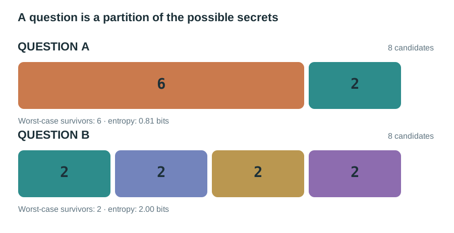
Guess A produces two outcomes, one compatible with six secrets and the other with two. Guess B produces four outcomes, each compatible with two. Both are valid questions, but guess B is more useful: no matter which answer the hidden code produces, at most two possibilities remain.
This picture captures almost the entire algorithm. An experiment is a function from possible secrets to possible answers. Asking the experiment tells you which preimage you are in. Good experiments partition the remaining possibilities into smaller groups.
Let \(S\) be the set of candidates and \(g\) a potential guess. For every possible response \(r\), define the bucket
\[ S_{g,r}=\{s\in S:F(s,g)=r\}. \]
The buckets are disjoint and together cover \(S\). For a deterministic feedback function, each secret produces precisely one bucket. Selecting the next question means comparing these partitions.
There are two natural ways to define “better”: protect yourself against the worst possible answer, or optimize for what happens on average.
2. Strategy one: protect against the worst case
You have no control over the hidden code, so you might want a guarantee. Consider the largest bucket produced by a guess. That is the number of candidates that could remain if you receive the least helpful answer.
The worst-case size of a guess is
\[ M(g)=\max_r|S_{g,r}|. \]
Choose the guess with the smallest \(M(g)\):
\[ g_{\mathrm{minimax}}=\arg\min_g\max_r|S_{g,r}|. \]
That is the minimax principle: minimize a quantity chosen by a hypothetical adversary who always gives you the least helpful valid answer. For the eight-code picture, A scores 6 and B scores 2. Minimax chooses B.
You do not need game-theory vocabulary to understand it. Imagine preparing for the most annoying answer you could receive. How much uncertainty would be left? Now choose the guess that makes this worst case as small as possible.
The surprising power of an impossible guess
A subtle point: the best test need not be a code that could still be the secret. A guess outside the surviving set can distinguish candidates especially well. In that case the guess cannot win immediately; it acts as a diagnostic experiment.
This is not merely theoretical. Donald Knuth’s classic analysis gives a situation in which using a code that is not among the remaining candidates is needed to retain his five-move guarantee. His paper explains this explicitly. The lesson is general: the best question is not always the most plausible answer.
A solver therefore needs two distinct sets:
- The surviving secret hypotheses \(S\)—what the answer might be.
- The allowed probes \(G\)—what guesses you are permitted to submit.
Restricting probes to \(S\) is an understandable optimization, but it can rule out more informative experiments.
3. Strategy two: optimize expected information
Minimax deliberately ignores how likely the different answers are. If one terrible response is extraordinarily unlikely, perhaps we are willing to tolerate it in exchange for better typical performance.
To formalize that idea, begin with a simpler question: What does it mean to be surprised by an answer?
If an event has probability \(p\), a natural measure of its information is
\[ I(r)=-\log_2p(r). \]
Why this formula? If an event has probability \(1/2\), observing it gives 1 bit. If it has probability \(1/4\), it gives 2 bits. If two independent events occur together, their probabilities multiply, while their information should add. Logarithms have exactly the required property: \(-\log_2(pq)=-\log_2p-\log_2q\).
An answer with probability 1 tells you nothing new: \(-\log_2(1)=0\). A rare answer, when it occurs, is highly informative.
But we must choose a question before seeing its answer. Therefore, we average the surprise over the possible responses. This is Shannon entropy:
\[ H(R_g)=-\sum_r p(r\mid g)\log_2p(r\mid g). \]
For uniformly probable candidate secrets and deterministic feedback, the probability of a response is simply its bucket’s relative size:
\[ p(r\mid g)=\frac{|S_{g,r}|}{|S|}. \]
In our eight-secret example, question A has distribution \((6/8,2/8)=(0.75,0.25)\), giving
\[ H(A)=-0.75\log_2(0.75)-0.25\log_2(0.25) \approx0.811\text{ bits}. \]
Question B has four equiprobable outcomes, so \(H(B)=2\) bits. B is the better question by this criterion, too.
Expected information is not the same as expected bucket size
Another popular score is the average number of surviving hypotheses:
\[ \mathbb{E}[|S_{g,R}|]=\sum_r p(r\mid g)|S_{g,r}|. \]
With a uniform prior this becomes \(\sum_r|S_{g,r}|^2/|S|\). Entropy and expected bucket size both reward good partitions, but they are different objective functions and can rank guesses differently. Neither one is guaranteed to minimize the total number of future guesses, because each looks only one step ahead.
Try the live strategy explorer. Each candidate guess is evaluated against every secret in a small space. Pick a guess manually, inspect its response buckets, or ask the program for the best minimax, entropy, or expected-size guess. The score is computed from the same feedback engine used in the first article.
4. The feedback algorithm has not changed
For ordinary Mastermind, a code has four slots and six available colors. We may encode the colors as 1 through 6; repetitions are allowed. This produces
\[ |\Omega|=6^4=1296 \]
possible secrets. When the secret is 2532 and the guess is 3523, the feedback is one exact match and two misplaced matches. The total matching symbols must be counted with multiplicity, not by distinct symbol membership.
Here is the core loop behind the question-selection algorithm:
function partition(candidates, guess, feedback) {
    const groups = new Map();
    for (const secret of candidates) {
        const response = JSON.stringify(feedback(secret, guess));
        if (!groups.has(response)) groups.set(response, []);
        groups.get(response).push(secret);
    }
    return [...groups.values()];
}

function minimaxGuess(candidates, allowedGuesses, feedback) {
    let bestGuess = null, bestWorst = Infinity;
    for (const guess of allowedGuesses) {
        const groups = partition(candidates, guess, feedback);
        const worst = Math.max(...groups.map(group => group.length));
        if (worst < bestWorst) {
            bestGuess = guess;
            bestWorst = worst;
        }
    }
    return bestGuess;
}
A practical implementation also needs a tie-breaker, a stopping condition, and—in larger code spaces—an efficient way to avoid evaluating every code against every possible guess. The strategy lab below makes these choices explicit and compares the three unweighted objectives on a complete, small code space.
Knuth’s five-guess algorithm
In The Computer as Master Mind (published in Journal of Recreational Mathematics, vol. 9(1), 1976–77), Donald Knuth showed a strategy that identifies every classic four-slot/six-color code in at most five guesses. His construction starts with 1122, evaluates candidate partitions, chooses a probe minimizing the largest remaining group, and prefers a still-possible solution when two probes have equally good scores. The complete construction matters: “use minimax” by itself is not a proof that every variant and every tie-break has a five-move guarantee.
The opening 1122 is revealing. Why begin with a repeated pair rather than four different colors? Because we are not maximizing how varied the guess looks. We are maximizing the usefulness of its possible responses. The partition structure, not our aesthetic sense of diversity, decides which experiment is good.
5. Play the algorithm
This local, browser-based lab implements classic Mastermind and two variants based on RAW Codebreaker. It invents a secret in your browser, gives feedback after each guess, filters the possible secrets, and can suggest a next probe.
For classic Mastermind the recommendation can inspect the complete 1,296-code universe. For the five-digit variants, ranking all 30,240 or 100,000 possible guesses against all possible secrets would be expensive in an interactive page. To remain responsive, the applet evaluates a sample of possible secrets and probes and labels those recommendations as approximate. The exact feedback and candidate filtering are never sampled.
6. RAW Codebreaker: more informative feedback, larger spaces
The RAW Codebreaker game changes the rules in an instructive way. Its code has five decimal positions and may begin with zero. Levels 1–3 use five distinct digits, giving
\[ 10\cdot9\cdot8\cdot7\cdot6=30{,}240 \]
possible secrets. Levels 4–6 permit repetitions, giving \(10^5=100{,}000\) possibilities. The attempt limits are 8, 7 and 6 in each set of three levels.
Mastermind reports two aggregate numbers. Codebreaker instead displays one colored clue per position: green means correct slot; amber means a present digit in another slot; gray means absent or a superfluous copy of a repeated digit. That positional information can distinguish secrets that would produce the same aggregate Mastermind feedback.
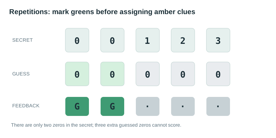
Repeated digits matter enormously. If the secret is 00123 and the guess is 00000, there are only two matching copies of zero. A correct implementation first allocates green exact matches. It then uses the remaining unmatched inventory to allocate amber matches. Any surplus guess copies must be gray.
Our local solver uses a deterministic left-to-right allocation of amber matches after greens. The published Codebreaker rules confirm the meaning of green, amber, gray and the treatment of surplus copies, but do not specify how amber marks are assigned when multiple copies compete for the same available digit. For direct integration with the server, that tie-breaking detail should be verified against its actual feedback implementation. This caution does not affect the classic Mastermind solver or the mathematical principles.
There is a further computational twist: feedback is still easy to calculate for any one guess, but the space of possible questions is now enormous. The interesting challenge shifts from filtering to efficient experimental design. Possible solutions include intelligent probe candidate selection, equivalence-class reductions, caching feedback, branch-and-bound, parallel evaluation, and approximation with explicit error checks.
7. Information has a prior: Bayesian Mastermind
Up to now we have treated every remaining code as equally likely. That is a prior assumption, not a property of Mastermind itself. If the secret generator samples uniformly at random, the assumption is justified. If a human selects a PIN, the prior may be extremely nonuniform: 0000, 1234 and birthdays may receive far more probability than arbitrary strings.
Instead of a set of survivors, maintain a probability distribution \(P(S=s)\). A new reported response \(r\) to guess \(g\) produces
\[ P(s\mid r,g)=\frac{P(r\mid s,g)P(s)}{\sum_u P(r\mid u,g)P(u)}. \]
With noiseless feedback, a wrong prediction has likelihood zero and a correct prediction has likelihood one. Thus Bayesian inference collapses to ordinary filtering, except that surviving candidates retain their relative prior weights. With a uniform prior it is literally the same operation as the constraint solver.
The strategic improvement is to evaluate possible answers using probability mass, not just candidate counts. For a deterministic question,
\[ p(r\mid g)=\sum_{s:F(s,g)=r}P(s). \]
A bucket containing four low-probability codes might matter less than a bucket containing one overwhelmingly likely code. A Bayesian information-gain policy chooses
\[ g^*=\arg\max_g I(S;R_g), \]
where \(I(S;R_g)\) is the mutual information between the secret and the observed answer to guess \(g\).
Why is this more than a fancy label? Because it tells us what we should optimize. We want to reduce our uncertainty about the secret, not necessarily the number of codes printed on a screen. If one code already carries probability 95%, spending a question distinguishing three unlikely alternatives may be less valuable than confirming or rejecting the dominant hypothesis.
8. What if the clues themselves are noisy?
Now make the problem more realistic. Suppose a person sometimes misreports a clue, a sensor occasionally produces an erroneous reading, or a communication channel corrupts one colored field. With hard constraints, a single false hint could eliminate the true code forever. A Bayesian solver can instead assign a small, nonzero likelihood to incorrect observations.
Bayes’ rule remains unchanged; only the likelihood model differs. Two useful examples are a symmetric categorical error model for whole responses and an independent per-slot color error model for Codebreaker-style reports. These are deliberately explicit mathematical assumptions; they are not claims that the real game makes errors.
In the noisy setting there is a subtle difference between entropy of the answer and information about the secret. The exact identity is
\[ I(S;R_g)=H(R_g)-H(R_g\mid S). \]
Here \(H(R_g\mid S)\) measures the variability of the reported answer even when the secret is known. That variability is noise, not information about the unknown code. A sensor that returns a random answer can have high output entropy while teaching you precisely nothing.
For noiseless deterministic feedback, \(H(R_g\mid S)=0\), so maximizing response entropy is the same as maximizing mutual information. When the observation model depends on the chosen experiment or is noisy, the distinction becomes essential.
This connects directly to Bayesian experimental design: use your current posterior distribution, predict the possible noisy observations for each proposed experiment, calculate the expected reduction in posterior entropy, then choose the most informative experiment. After receiving its answer, update the posterior and repeat.
9. Is greedy information gain actually optimal?
It is easy to say “always maximize entropy,” but what exactly is the objective? There are several different optimization problems hiding under the word optimal.
Minimax minimizes the maximum number of candidates surviving the next answer. Entropy maximizes expected information from the next answer. Expected-size minimizes the expected number of candidates surviving the next answer. Expected-turns seeks the smallest expected number of guesses until victory, potentially considering many steps ahead. These objectives generally differ.
For full-game optimization, we would ideally construct a decision tree. Each node chooses a guess. Each branch corresponds to a possible feedback value. Each leaf corresponds to winning on a secret. We can define a recursive cost-to-go:
\[ V(S)=\min_{g\in G}\Bigl[1+\sum_{r\ne\text{win}}p(r\mid g)\,V(S_{g,r})\Bigr], \]
with a sensible terminal condition for an already solved secret and with branches that cannot improve excluded. In a weighted Bayesian version, \(S\) also carries posterior probabilities. The recursion makes clear why looking one step ahead may fail: two guesses with similar immediate partitions can lead to subproblems of very different difficulty.
This dynamic program is conceptually straightforward but computationally expensive because the state is an entire belief distribution or survivor set. There can be exponentially many distinct states. That is why excellent practical solvers often use greedy partition metrics, memoization, bounded search and domain-specific symmetry reductions.
Measure strategies instead of guessing which is best
The benchmark below solves every secret in a deliberately small Mastermind universe: three positions, three symbols, repetitions allowed (\(3^3=27\) secrets). The results are actual runs of the shared solver. For each strategy, we show the mean and worst number of guesses, counting the final successful guess. This is not a benchmark of classical four-slot Mastermind and it should not be presented as one.
The benchmark teaches an important discipline: state the configuration, distribution over secrets, available guesses, feedback convention and tie-breaker before comparing algorithms. Otherwise, apparently contradictory performance claims may simply describe different games.
10. A general algorithm for scientific experiments
The connection extends far beyond code puzzles. Replace the secret code with an unknown physical model, a software defect, a disease hypothesis, or a hidden system parameter. Replace a guess with an experiment or diagnostic test. Replace colored pegs with the resulting observation.
The mathematical cycle stays the same:
- Define a hypothesis space and your current beliefs.
- Predict what each candidate experiment would report under each hypothesis.
- Choose an experiment according to an explicit objective: worst-case resolution, expected information, financial cost, time or safety.
- Observe the result and update the possible hypotheses or their posterior probabilities.
- Repeat until the evidence is sufficient to act.
In a deterministic code puzzle, every hypothesis predicts a perfect answer. In the real world, likelihoods often represent measurement error and intrinsic variation. The Bayesian formulation therefore generalizes naturally, while the simple constraint solver becomes an important special case.
The deepest lesson is perhaps this: intelligence is not only finding the right answer from the information you have. It is learning to choose the information worth acquiring next.
The companion article derives the feedback function, solves 682/614/206/738/380 by logic and exhaustive filtering, and shows how deterministic filtering fits into Bayesian inference.
Read the constraint-solving article →References
- [Shannon1948]Shannon, C. E. (1948). “A Mathematical Theory of Communication.” Bell System Technical Journal, 27(3), 379–423. doi:10.1002/j.1538-7305.1948.tb01338.x.
- [Knuth1976]Knuth, D. E. (1976–77). “The Computer as Master Mind.” Journal of Recreational Mathematics, 9(1). Paper.
- [RAWCodebreaker]RAW Codebreaker. Public rules for the five-digit, six-level positional-feedback variant.
The interactive Mastermind and Codebreaker games on this page use randomly generated local secrets, not a connection to the official daily Codebreaker service. The two-site feedback allocation models should not be conflated without checking server behavior.